Houdini Procedural Explosion VFX

01 Breakdown — System Philosophy

This Houdini procedural explosion VFX setup is built as a deterministic, layer-based system designed for simulation accuracy and export flexibility.

What I find genuinely interesting in VFX work is not any single effect — it's the patterns underneath. Most effects, when you look closely enough, share the same structural logic. Find that logic, build a system around it, and you get something reusable, predictable, and fast to iterate.

Fig 01: Unity Explosion VFX — real-time playback from VAT export.

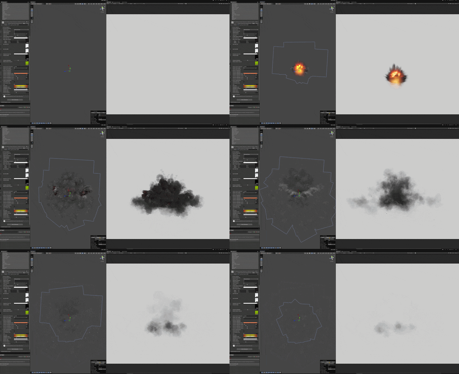
This breakdown is about that process — using a procedural explosion as the example. Not because explosions are unique, but because they're a good stress test: clear physical reference, multiple simultaneous layers, and they need to work across very different rendering contexts. Getting all of that into one coherent system requires thinking about architecture first and aesthetics second.

Gallery 01: Simulation stages — burst expansion, layer composition, final look.

02 Before Opening Houdini: Scale and Reference

The first thing I do before touching any node is establish ground truth — physically correct scene scale and a solid visual reference.

Scale matters more than most people realize. In Houdini's geometry context (SOPs), units are dimensionless — one unit can mean anything. But the moment you move into simulation (DOPs), everything changes. Pyro, RBD, and FLIP solvers operate on MKS units: meters, kilograms, seconds. Gravity, viscosity, density, buoyancy — all calculated against real physical values.

For reference, I used real footage of a 122mm high-explosive artillery shell detonation. Any VFX effect is a combination of static shape and animation. Break it into layers and you get: flame, smoke, debris, displaced ground, shockwave, crater. There's an impact, a detonation, an active expansion phase, and a decay.

These patterns — extracted from reference — became the architecture of the tool.

Fig 02: Reference analysis — phase extraction becomes HDA architecture.

03 HDA Architecture: The Pipeline

I built the system as two connected HDAs to separate geometry generation from heavy simulation data. This creates a clean, debuggable workflow.

Layer-Based Organization

At a high level, an explosion is smoke, fire, and fragments. Each layer is independent and operates on its own geometry, velocity field, and timing:

04 HDA 1: Initial Mesh and Velocity

Everything starts with two objects: a sphere defines the shape and scale of the explosion, and a point defines the direction. These are the two inputs to the first HDA. From there, the configuration is managed via three primary tabs.

Fig 04: HDA 1 — Initial Mesh Setup Interface. Three-tab structure.

Tab 1: Initial Shape

This tab controls the base geometry from which velocity is calculated. A turbulent Perlin noise is applied to the sphere, creating the characteristic spikes radiating from the epicenter visible in the first frames of any real explosion.

The noise is masked through the dot product of the mesh normals: near the ground, the shape automatically smooths out. This is physically correct — the blast wave flattens as it meets surface resistance.

Fig 04a: Perlin noise masked by normal dot product — ground contact smooths automatically.

A separate parameter — Point Direction Interpolation (Bias) — interpolates between the original point position and the reference direction point (second input). At Bias = 0, the explosion is symmetric. Offset it and you get a directional blast matching the shell's angle of entry. No manual geometry editing required.

Fig 04c: Flow Noise layer can be enabled on top for additional organic variation.

Tab 2: Burst Animation

This tab controls how the explosion lives in time.

Fig 04d: Burst Animation tab — dual curve control for temporal shape.

Tab 3: Layers

This is where the core logic lives. The current setup has 4 layers, each independent.

Gallery 04: Four independent layers — Main Burst / Curl / Shockwave / Pump.

The debris section is separate from the main layers. Points scatter per fragment, additional vertical velocity is added, Curl Noise controls trajectory variation, and a Spinning Force range drives per-fragment random rotation.

Gallery 04b: Debris system — fragment scatter with Curl trajectory and spin.

05 HDA 2: Rasterization and Pyro

The second HDA receives the data from the first. On initialization, a Python script reads the layer count and types from HDA 1 and auto-configures the interface — the designer gets a ready-made interface that matches whatever was set up upstream.

Fig 05: se_simulation DOP network — LAYERS / DEBRIS / PUMP / SIM branches auto-built by Python.

The system programmatically builds the DOP network, ensuring simulation setup is always in sync with geometry sourcing:

# =============================================================================
# DOP NODE CREATION — auto-builds Volume Source nodes from HDA 1 layer config
# =============================================================================

def create_dop_volume_source_nodes():
    """Creates and configures all Volume Source nodes in the DOP network."""
    log("\n--- Updating DOP Volume Source Nodes ---")
    node = hou.pwd()

    try:
        dop_network = node.node("sim_explosion")
        if not dop_network:
            log("DOP Network 'sim_explosion' not found.", "ERROR")
            return

        merge_node  = dop_network.node("merge1")
        switch_node = dop_network.node("switch1")  # may be None

        _configure_smoke_object(dop_network)

        # Iterate DOP_CONFIGS — one entry per layer type (burst/debris/pump)
        for config in DOP_CONFIGS:
            config_func = globals()[config["config_func"]]
            _create_or_update_dop_sources(
                parent_node    = node,
                dop_network    = dop_network,
                merge_node     = merge_node,
                switch_node    = switch_node,
                count_parm_name= config["count_parm"],
                source_prefix  = config["source_prefix"],
                null_prefix    = config["null_prefix"],
                config_func    = config_func
            )

        dop_network.layoutChildren()

    except Exception as e:
        log(f"Error in create_dop_volume_source_nodes: {e}", "ERROR")
        import traceback
        traceback.print_exc()

Tab 1: Pyro Setup — Noise per Layer

Per-layer noise settings for density and temperature — type, frequency, detail. This is where the character of the smoke is defined: how lumpy, how uniform, how the edges behave.

For the main burst layer: Alligator noise — it produces the characteristic bumpy structure close to how real smoke behaves at cloud boundaries. The Debris layer has a separate Velocity tab with optional Curl Noise for additional swirl along fragment trajectories.

Fig 05a: Pyro Setup tab — per-layer noise configuration.

Tab 2: Rasterize Attributes

Controls how the point cloud is converted into a VDB volume. Each layer has a Particle Scale — the influence radius of each point during rasterization.

Fig 05b: Rasterize Attributes — particle scale per layer.

Tab 3: Smoke Simulation

Pyro solver settings. Voxel Size balances detail against simulation time. Per-layer multipliers for Density, Temperature, and Velocity determine the weight of each layer in the final simulation. The shockwave and curl layers get a higher velocity multiplier to amplify their influence on smoke behavior.

Fig 05c: Smoke Simulation tab — voxel size and per-layer multipliers.

06 R&D & Validation: Pipeline Tests

Verification is critical in a procedural pipeline. Before locking the HDA logic, I ran iterative tests to validate velocity field behavior, layer blending, and rendering fidelity in Arnold.

1. Initial Mesh Velocity & Noise

Validating procedural noise distribution before rasterization. This test ensures the velocity vectors match the desired explosive expansion patterns — if they don't, fixing it here costs seconds, not hours of sim cache.

2. Volume Layers Blend

Testing the interaction between independent layers (Burst, Curl, Shockwave, Pump). The system must handle volume density blending at the boundaries to prevent clipping or artifacting.

3. Arnold Render Test

Final validation. Using a 1 Camera AA pass, we verify that the VDB volumes generated by the simulation hold up to light absorption, scattering, and motion blur in the renderer.

07 Export: The Engine Doesn't Matter

After simulation, the output is exported in whatever format the pipeline requires. The engine doesn't matter because all the physics and shape were determined at the point animation stage — by the time you export, it's data, not logic.

The same setup delivers cinematic renders and real-time game effects. The fundamentals are always the same. Only the output format changes.

08 Camera Setup

Camera configuration is often overlooked but it directly affects both render time and export quality — and the setup is completely different depending on your target.

Gallery 08: Houdini VAT export orthographic camera configuration.

09 Motion Vectors — Frame Blending

Motion Vector texture stores the per-pixel direction and magnitude of movement between frames. In a game engine, the shader uses this data to interpolate between flipbook frames at runtime — effectively faking in-between frames that were never rendered.

Without Motion Vectors, a flipbook plays as a hard cut between frames — stutter is clearly visible, especially at low frame counts. With Motion Vectors enabled, the engine blends between frames based on actual movement direction, so 16 or 24 rendered frames can look as smooth as 60. This directly reduces texture memory and render time without sacrificing perceived quality.

Fig 09: Frame Blending — standard flipbook stutter vs. Motion Vector interpolation.

10 Six Point Lighting — Real-Time Integration

Standard sprite or flipbook effects are lit as flat surfaces — they receive light from one direction and ignore everything else. This looks fine in a static scene but breaks the moment a dynamic light source moves, or the effect is placed near colored environment lighting.

Fig 10a: Six Point Lighting — flat billboard vs. dynamic environment response.

Six Point Lighting solves this. During the Houdini render, six separate cameras capture the volume from six directions — Top, Left, Right, Bottom, Back, Front. The resulting two textures (TLR and BBF) store baked illumination for each voxel from all six axes.

In-engine, the shader reconstructs approximate volumetric lighting by blending these six samples based on the current light direction. The explosion responds correctly to any light in the scene — a muzzle flash nearby, rotating sunlight, colored fill from an environment — without any volumetric rendering, without runtime simulation.

Fig 10b: Houdini — Six Point Lighting render preparation, six-camera rig setup.